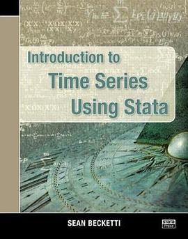
Introduction to Time Series Using Stata pdf epub mobi txt 电子书 下载 2025

想要找书就要到 图书目录大全

立刻按 ctrl+D收藏本页

你会得到大惊喜!!

Recent decades have witnessed explosive growth in new and powerful tools for timeseries analysis. These innovations have overturned older approaches to forecasting, macroeconomic policy analysis, the study of productivity and long-run economic growth, and the trading of financial assets. Familiarity with these new tools on time series is an essential skill for statisticians, econometricians, and applied researchers.

Introduction to Time Series Using Stata provides a step-by-step guide to essential timeseries techniques from the incredibly simple to the quite complex and, at the same time, demonstrates how these techniques can be applied in the Stata statistical package. The emphasis is on an understanding of the intuition underlying theoretical innovations and an ability to apply them. Real-world examples illustrate the application of each concept as it is introduced, and care is taken to highlight the pitfalls, as well as the power, of each new tool.

Sean Becketti is a financial industry veteran with three decades of experience in academics, government, and private industry. Over the last two decades, Becketti has led proprietary research teams at several leading financial firms, responsible for the models underlying the valuation, hedging, and relative value analysis of some of the largest fixed-income portfolios in the world.

Table of contentsList of tables
List of figures
Preface
Acknowledgments
1 Just enough Stata
1.1 Getting started
1.1.1 Action first, explanation later
1.1.2 Now some explanation
1.1.3 Navigating the interface
1.1.4 The gestalt of Stata
1.1.5 The parts of Stata speech
1.2 All about data
1.3 Looking at data
1.4 Statistics
1.4.1 Basics
1.4.2 Estimation
1.5 Odds and ends
1.6 Making a date
1.6.1 How to look good
1.6.2 Transformers
1.7 Typing dates and date variables
1.8 Looking ahead
2 Just enough statistics
2.1 Random variables and their moments
2.2 Hypothesis tests
2.3 Linear regression
2.3.1 Ordinary least squares
2.3.2 Instrumental variables
2.3.3 FGLS
2.4 Multiple-equation models
2.5 Time series
2.5.1 White noise, autocorrelation, and stationarity
2.5.2 ARMA models
3 Filtering time-series data
3.1 Preparing to analyze a time series
3.1.1 Questions for all types of data
How are the variables defined?
What is the relationship between the data and the phenomenon of interest?
Who compiled the data?
What processes generated the data?
3.1.2 Questions specifically for time-series data
What is the frequency of measurement?
Are the data seasonally adjusted?
Are the data revised?
3.2 The four components of a time series
Trend
Cycle
Seasonal
3.3 Some simple filters
3.3.1 Smoothing a trend
3.3.2 Smoothing a cycle
3.3.3 Smoothing a seasonal pattern
3.3.4 Smoothing real data
3.4 Additional filters
3.4.1 ma: Weighted moving averages
3.4.2 EWMAs
exponential: EWMAs
dexponential: Double-exponential moving averages
3.4.3 Holt–Winters smoothers
hwinters: Holt–Winters smoothers without a seasonal component
shwinters: Holt–Winters smoothers including a seasonal component
3.5 Points to remember
4 A first pass at forecasting
4.1 Forecast fundamentals
4.1.1 Types of forecasts
4.1.2 Measuring the quality of a forecast
4.1.3 Elements of a forecast
4.2 Filters that forecast
4.2.1 Forecasts based on EWMAs
4.2.2 Forecasting a trending series with a seasonal component
4.3 Points to remember
4.4 Looking ahead
5 Autocorrelated disturbances
5.1 Autocorrelation
5.1.1 Example: Mortgage rates
5.2 Regression models with autocorrelated disturbances
5.2.1 First-order autocorrelation
5.2.2 Example: Mortgage rates (cont.)
5.3 Testing for autocorrelation
5.3.1 Other tests
5.4 Estimation with first-order autocorrelated data
5.4.1 Model 1: Strictly exogenous regressors and autocorrelated disturbances
The OLS strategy
The transformation strategy
The FGLS strategy
Comparison of estimates of model
5.4.2 Model 2: A lagged dependent variable and i.i.d. errors
5.4.3 Model 3: A lagged dependent variable with AR(1) errors
The transformation strategy
The IV strategy
5.5 Estimating the mortgage rate equation
5.6 Points to remember
6 Univariate time-series models
6.1 The general linear process
6.2 Lag polynomials: Notation or prestidigitation?
6.3 The ARMA model
6.4 Stationarity and invertibility
6.5 What can ARMA models do?
6.6 Points to remember
6.7 Looking ahead
7 Modeling a real-world time series
7.1 Getting ready to model a time series
7.2 The Box–Jenkins approach
7.3 Specifying an ARMA model
7.3.1 Step 1: Induce stationarity (ARMA becomes ARIMA)
7.3.2 Step 2: Mind your p’s and q’s
7.4 Estimation
7.5 Looking for trouble: Model diagnostic checking
7.5.1 Overfitting
7.5.2 Tests of the residuals
7.6 Forecasting with ARIMA models
7.7 Comparing forecasts
7.8 Points to remember
7.9 What have we learned so far?
7.10 Looking ahead
8 Time-varying volatility
8.1 Examples of time-varying volatility
8.2 ARCH: A model of time-varying volatility
8.3 Extensions to the ARCH model
8.3.1 GARCH: Limiting the order of the model
8.3.2 Other extensions
Asymmetric responses to “news”
Variations in volatility affect the mean of the observable series
Nonnormal errors
Odds and ends
8.4 Points to remember
9 Models of multiple time series
9.1 Vector autoregressions
9.1.1 Three types of VARs
9.2 A VAR of the U.S. macroeconomy
9.2.1 Using Stata to estimate a reduced-form VAR
9.2.2 Testing a VAR for stationarity
Other tests
9.2.3 Forecasting
Evaluating a VAR forecast
9.3 Who’s on first?
9.3.1 Cross correlations
9.3.2 Summarizing temporal relationships in a VAR
Granger causality
How to impose order
FEVDs
Using Stata to calculate IRFs and FEVDs
9.4 SVARs
9.4.1 Examples of a short-run SVAR
9.4.2 Examples of a long-run SVAR
9.5 Points to remember
9.6 Looking ahead
10 Models of nonstationary time series
10.1 Trends and unit roots
10.2 Testing for unit roots
10.3 Cointegration: Looking for a long-term relationship
10.4 Cointegrating relationships and VECMs
10.4.1 Deterministic components in the VECM
10.5 From intuition to VECM: An example
Step 1: Confirm the unit root
Step 2: Identify the number of lags
Step 3: Identify the number of cointegrating relationships
Step 4: Fit a VECM
Step 5: Test for stability and white-noise residuals
Step 6: Review the model implications for reasonableness
10.6 Points to remember
10.7 Looking ahead
11 Closing observations
11.1 Making sense of it all
11.2 What did we miss?
11.2.1 Advanced time-series topics
11.2.2 Additional Stata time-series features
Data management tools and utilities
Univariate models
Multivariate models
11.3 Farewell
References
Author index
Subject index
· · · · · · (收起)